While the proliferation in the amount of data modern businesses collect has created many opportunities, it has also introduced challenges for sound decision-making. In some organizations, earnest efforts to be “data-driven” devolve into a culture of false certainty in which the influence of metrics is dictated not by their reliability but rather by their abundance and the confidence with which they’re wielded.
For example, in the paid marketing domain, practitioners have unprecedented access to data about who clicked on what ads and converted when. Most companies use these data to drive decisions about millions (or even billions) of dollars: quantifying advertising channel or campaign performance, making changes to marketing campaigns, and constructing attribution metrics that assign credit to advertisements based on whether a new customer clicked on them before converting. The ability to slice and dice these data has given the impression of visibility into performance at any level of granularity.
Unfortunately, it’s often only an impression. Looking at more data on more things doesn’t necessarily produce better decisions; in many cases, it actually leads to worse ones.
What’s a decision, anyway?
Decisions are about choosing between different sets of actions. The right decision is simply the one that, among the set of alternatives, would bring about, or cause, the best outcome.
\[d_{opt} = \arg\max\limits_{d \in D} U(\cal{f}(d))\]As implied by the formulation above, decision-making is trivial when the candidate outcomes are known in advance, here indicated as \(f(d)\) plugged into utility function, \(U\). The real challenge (and opportunity) is in obtaining accurate estimates of what these outcomes might be. Enter, data!
If there’s one thing data scientists are good at, it’s throwing a bunch of data into XGBoost and estimating \(\mathbb{E}(Y \mid X)\). Decisions, however, rely on a very special kind of estimate—one that tells us about the outcome we’d observe if we intervened on the world by enacting decision \(d\), aka the potential outcome.
Let’s pretend that you want to cut down on unnecessary medicine. You have a headache and are trying to decide whether or not to take ibuprofen. To guarantee the right decision, you’ll need to know the relevant potential outcomes: whether you’ll recover from the headache in less than an hour if you take ibuprofen, \(Y_{d=i}\), and whether you will recover if you don’t take ibuprofen, \(Y_{d=\neg i}\). If \(Y_{d=i}=1\), indicating that the headache will go away in less than an hour if ibuprofen is taken, and \(Y_{d=\neg i}=0\), that it won’t otherwise, then taking ibuprofen is the right decision; any other potential outcome configuration (e.g, \(Y_{d=i}, Y_{d=\neg i} = 1\)) would make not taking ibuprofen the best option.
As a dogged empiricist, you’ve actually collected data on this. In fact, for the last two years, you’ve recorded every headache, indicated if you took ibuprofen and whether the headache subsided within an hour. Your dataset looks like this:
| Day | Took ibuprofen? | Recovered? | $$Y_{d=i}$$ | $$Y_{d=\neg i}$$ |
|---|---|---|---|---|
| 1 | 1 | 1 | 1 | Null |
| 14 | 0 | 1 | Null | 1 |
| ... | ... | ... | ... | ... |
| 719 | 1 | 0 | 0 | Null |
Notice the abundance of missing values in the potential outcomes columns. Sadly, you can only observe one potential outcome at a time. For example, if you wanted to fill in the missing value for \(Y_{d=\neg i}\) on day 1, you’d literally need to travel back in time and not take ibuprofen to observe it. Absent a time machine, how might you use this null-value ridden data to estimate the future values \(Y_{d=i}\) and \(Y_{d=\neg i}\) and decide whether or not to take ibuprofen now?
With a time machine, you could fill in these null values and calculate \(\mathbb{E}(Y_{d = i}) - \mathbb{E}(Y_{d = \neg i})\), which would tell you how frequently ibuprofen caused or would have caused you to recover in the last two years. Further, such quantities might make for great potential outcome estimates of your current decision (e.g., \(\hat{Y}_{d = i} = \mathbb{E}(Y_{d = i})\)) [1].
One set of questions these data can answer is on average, what percent of the time you recovered from a headache with ibuprofen, \(\mathbb{E}(Y_{d = i} \mid d=i)\) and without, \(\mathbb{E}(Y_{d=\neg i} \mid d=\neg i)\). You could use these averages as potential outcome estimates of taking vs. not taking ibuprofen, but would they be any good? For example, it may be the case that you only take ibuprofen when your headache is very severe and conversely, forgo it when the headache seems to be dissipating on its own. A naive comparison might even suggest that ibuprofen has made recovery less likely.
Fortunately, the field of causal inference tells us how to make such estimates along with what data and assumptions are required to do it well. That means that if we’re thoughtful (and lucky), we may not actually need a time machine to produce good estimates of \(\mathbb{E}(Y_{d})\) and put them to good use as estimates for the potential outcomes of the decision we’d like to inform. When we talk about potential outcomes under different decision rules, \(Y_d : d \in D\), we’re talking about the causal relationships between our decisions and outcomes. The better our understanding of those causal relationships, the better decisions we’re likely to make. If our goal is to improve our understanding of causal relationships, more data is not necessarily better. In this context, data is only valuable if it improves our causal understanding.
Causality
“Should I pay the Google Tax?” (This question is harder than you think)
In paid marketing, one major channel for many advertisers is Search Engine Marketing (SEM). Search ads are sponsored links associated with a user’s search term. Marketers use SEM to get their ads to appear at the top of search results for high-intent users. For example, if you’re hangry now, several companies will offer to solve your problem:

One decision within this channel is whether or not to spend money advertising to people who are already explicitly searching for your brand.
So-called branded keyword ads are the advertisements that appear in search results when you enter the name of a brand:

For businesses, branded search ads are irritating. It seems cosmically unfair to pay for people so obviously interested in one’s own brand or trademark. But not advertising to people who search for your brand means the ads of competitors appear first in the search results. Dubbed the Google Tax, branded-keyword search campaigns can result in an arms race among competing companies. Some companies address this via trademark complaint or informal agreements with competitors. This can result in a legal headache.
Before we summon the lawyers, let’s take a step back. Why pay for clicks on your brand’s keywords? A common rationale is that it’s an inexpensive way to immediately acquire clients. But consider an alternative narrative: might internet users searching for your brand be devoted enough to click on the organic results [2] just inches below the sponsored ones? If so, paying for branded keywords does not cause any net conversions since people were going to convert even if the ad didn’t appear. (This narrative is not as outlandish as it might seem, e.g. eBay.) In this case, there may be other rationales for paying the Google Tax, but “inexpensive acquisition” wouldn’t be one of them.
To be clear, paying the tax is fine as long as you know what you’re getting. Unfortunately, many companies don’t.
Before we decide to buy these ads, we’d like to ensure that they will actually cause people to sign up for our service that wouldn’t otherwise. This requires an understanding of the following potential outcomes: the number of clients we would acquire by spending \(x > 0\) on branded ads, which we’ll call \(Y_{1}\), and number we’d get by spending \(x = 0\), \(Y_{0}\). As in the ibuprofen example above, we can use our historical data to inform our expectations about these potential outcomes by asking whether, on average, buying paid ads caused people to sign up that wouldn’t have otherwise. With this question in mind, we can define our target parameter as, \(\psi_0^F = \mathbb{E}[Y_1] - \mathbb{E}[Y_0]\), which we’ll assume for this example implies \(U(f(1)) > U(f(0))\) if \(\psi_0^F > 0\).
Since we’ve bought such ads in the past, we might seek to inform these expected potential outcomes by looking at the number of customers who clicked on them before converting in the historical data. Alternatively, one could regress new customer counts on branded keyword ad spend. These strategies, however, would lead to poorly estimated expectations and likely very poor decisions.
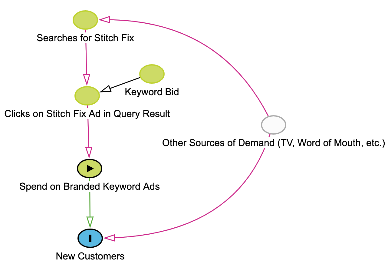
In this example, the causal relationship between ad spend and new customer acquisition is confounded by things like word of mouth, television ads, media coverage, etc. For example, when we run a television campaign, the number of people searching for “Stitch Fix” on Google to find our website increases. When a Stitch Fix ad appears at the top of their results, they often click it even if they would have visited our website anyway, causing our spend to increase on branded keywords without necessarily inducing additional people to visit our site that wouldn’t have otherwise. Independent of these searches, television campaigns can simultaneously cause an influx of new clients. This can result in a very strong association between branded keyword ad-spend and new client numbers—not because branded search ads are causing people to sign up—but because other sources of new customer demand (e.g., TV ads) may be a persistent, common cause of both.
Even with infinite data, the quality of such decisions will be very poor if we’re unable to understand the causal effects historically associated with one course of action versus another. In the example above, the regression parameters could completely misrepresent the effectiveness of branded search ads and lead to a highly inefficient allocation of advertising resources.
What is my data telling me?
We’ve all heard the platitude that correlation doesn’t imply causation, but sometimes it does! The process of understanding when it does is often referred to as causal identification. If a relationship between two variables is causally identified, it means we can directly estimate useful summaries (e.g., the expectations) of its potential outcomes from the data we have (despite the missing potential outcomes we could only observe with a time machine).
One of our favorite tools in this arena is causal Directed Acyclic Graphs (DAGs). DAGs are a powerful and intuitive tool for encoding causal assumptions about the data generating process of interest—in particular, whether the relationship we want to learn about is confounded by other phenomena. Nodes represent variables in our system while arrows indicate a directional causal connection. The biggest assumptions you make in a DAG are the nodes and arrows you leave out. Combined with a set of rules called the backdoor criterion and assumptions about consistency and positivity, which we won’t describe here, the DAG can help reveal whether and how causality can be established with the data at hand [3].
In the DAG pictured below, we are interested in the number of new customers we would acquire by adjusting the amount we spend on branded keyword ads. Unfortunately, there is another causal path with arrows pointing to both spend and new customer acquisition; this is known as a backdoor path and means that, unless we can block it, correlation does not imply causation and summaries of potential outcomes cannot be estimated directly from the data.

Though sometimes we may get lucky and be able to identify causal effects in observational data, randomized experiments are the tried and true way of identifying and estimating such effects. In the paid search example, if we randomize ad spend [4], it will become independent of any other cause, in contrast to the observational setting, where other sources of demand are a common cause (aka a confounder) of both spend and customer acquisition. In the context of our DAG, randomization blocks any backdoor paths between ad spend and new customers by deleting any arrows pointing to ad spend.
Can’t I just use XGBoost?
(Actually, yes! But hold on a minute, we’ll get there.)
The most common way of blocking a backdoor path is adjustment. As it turns out, our branded paid search DAG presents just such an opportunity! Assuming our DAG is correct [5] (and that positivity / consistency assumptions are also satisfied), adjusting for Stitch Fix searches will make the residual correlation between spend and new customer acquisition a causal one.
To adjust for Stitch Fix searches, we could estimate our expected potential outcomes with a simple weighted average:
\[\mathbb{E}[Y_d] = \sum_s \mathbb{E}[Y \mid Spend=d, Searches=s]P(Searches=s)\]However, in most settings, such an approach would suffer from data sparsity issues with respect to the variable we’re adjusting for—in this case, the number of searches for Stitch Fix.
Alternatively, we could specify \(\mathcal{Ye\,Olde\,Regression\,Model}\):
\[Y \sim N(\alpha_0 + spend \times \alpha_1 + searches \times \alpha_2, \sigma)\]Where \(\alpha_1\) would be our estimate of the target parameter. Since searches is a continuous variable, a linear relationship may be a very poor approximation—effectively the opposite problem from the weighted average estimator. In addition, even if the relationship is truly linear, OLS will yield inconsistent and biased estimates in the presence of treatment effect heterogeneity (which should always be the default assumption), even with infinite data!
For such problems at Stitch Fix, we turn to a semiparametric method from modern effect estimation called targeted maximum likelihood estimation (TMLE [6]). TMLE throws the kitchen sink at estimating \(P(Y \mid spend, searches)\) and \(P(spend=1 \mid searches)\) using an ensembling technique called Superlearner, which constructs a linear combination of any set of predictive / machine learning models (XGBoost is available in CV-TMLE, check out the link above) and weights them using cross validation, generally performing better in practice than any single model would. TMLE is also targeted, which means that instead of optimizing the performance of the whole prediction function, it focuses all its energy on estimating the target parameter of interest, \(\psi_0^F\), as well as possible. In addition, it’s double robust, which means that if either prediction function is correctly specified, TMLE’s estimate will converge to the right answer.
Conclusion
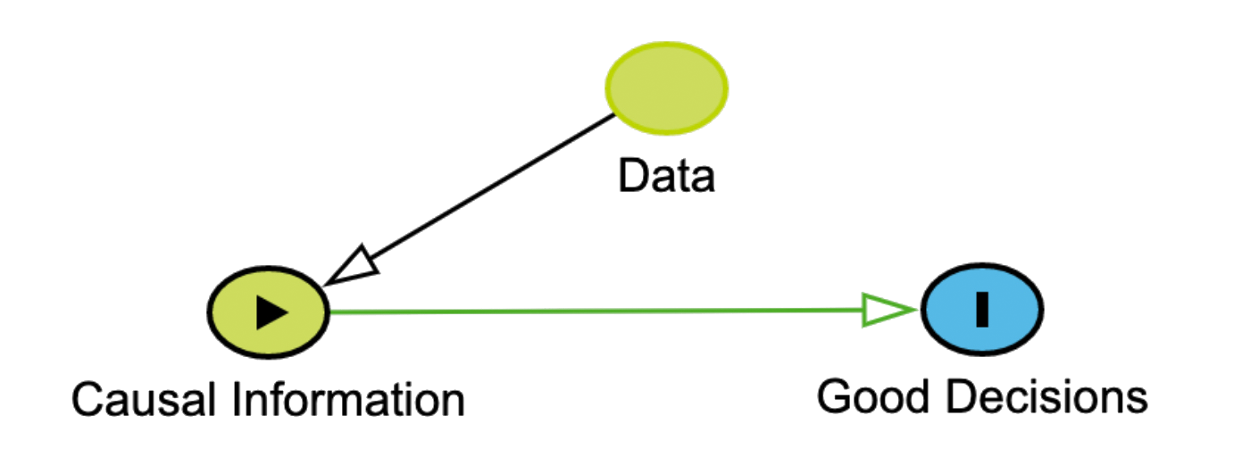
In summary, data can only improve decisions insofar as it enables us to learn about the potential outcomes associated with the alternatives under consideration. Instead of being naively data driven, we should seek to be causal information driven. Causal inference provides a set of powerful tools for understanding the extent to which causal relationships can be learned from the data we have. Standard machinery will often produce poor causal effect estimates, which modern methods from effect estimation, such as TMLE, will consistently outperform. By taking these considerations seriously at Stitch Fix, we foster a culture of better, clearer decision-making.
References
[1]↩ In this blog we limit our focus to cases where the past, present and future can all be assumed to have a common data generating distribution. There are situations where this may not be true. Interested readers may wish to consult literature on causal transportability to learn more.
[2]↩ The set of results returned by a given search that are not paid for by any advertiser.
[3]↩ Some of you may find our mixing of Rubin’s potential outcomes framework with Pearl’s nonparametric structural equation modeling framework a bit surprising, if not downright sacrilegious! At Stitch Fix, data scientists are incurable pragmatists: we find the potential outcomes framework to be a nice, intuitive way to introduce people to the concept of causality in statistics; AND we find DAGs to be an indispensable tool for expert elicitation during the causal identification process.
[4]↩ Note that in reality, ad spend can only be randomized through randomizing keyword bids.
[5]↩ This DAG is oversimplified for the sake of pedagogy. For a more detailed discussion of causal effect identification and estimation in paid search see this article by Google Research.
[6]↩ Here’s a nice introductory article on TMLE. There are implementations in both R and Python.
