Introduction
“Give me jeans not shoes.” That may seem like a simple request, but when we process that bit of text with our human brains, we take a lot for granted. The text is loaded with context that we parse effortlessly, thanks to a lifetime of language training (and some innate skills). Yet, it is surprisingly tricky to train a machine to do this.
At Stitch Fix, our main objective is to help our clients find the clothes they love. Our talented stylists give the highest priority to what clients ask for when requesting a Fix. Clients share invaluable information about their preferences and special requests, like finding a suitable outfit for a wedding or upcoming trip, in Fix Notes. They also mention what clothes they have enough of or what kinds of clothes they don’t imagine ever wearing. These examples only scratch the surface of how our clients interactively participate in the styling process by the use of Fix Notes. Extracting useful information from these notes is an extremely challenging task that warrants the use of sophisticated algorithms. In this post, we will explore how state-of-the-art Natural Language Processing (NLP) models aid us in carrying out this complicated task.
As you may know, NLP is one of the most challenging domains in artificial intelligence and machine learning, but recent advancements in NLP have led to some very promising results. BERT, an NLP model developed by Google, has achieved outstanding results on many NLP tasks1. By exploiting attention mechanisms, BERT comes up with dynamic representations (or embeddings) for each word in the input text based on the context these words appear in.
Objective
Our team’s new stylist selection algorithm has shown excellent performance in helping stylists pick the best items for our clients. To feed this model with input features, we need to extract information from many sources, including Fix Notes. A common place to start with NLP is the bag-of-words approach, but this doesn’t capture the contextual relationship between words, nor does it take into account word order. For example, “Give me jeans not shoes” and “Give me shoes not jeans” would receive the same representation with this approach. Our goal is to come up with features that bear more information about the requests so that our styling model can do a better job at clothing item selection. This is where we get help from attention-based NLP models. Throughout this post, we will discuss the basic operations behind BERT in the hopes of familiarizing data scientists and other interested readers with these models and their potential applications in addressing similar problems.
Attention-Based NLP Models
You might have heard about the controversial OpenAI language model that generates long, coherent paragraphs of text given an initial prompt. (Give it a try here.) This language-generation model is based on an attention-based model called Transformer. (BERT is also a Transformer.) In this post, we will build upon simple concepts to learn first what attention is, and then gradually transition through the hierarchy to construct Transformers and then BERT.
Consider this client request: “Give me jeans not shoes.” In order to represent this sentence as a high-dimensional vector, we have several options, some of which come up with a fixed high-dimensional representation (embedding) for each word in the input sentence. You can read more about word embeddings in this post. The problem with fixed word embeddings is that they don’t capture the true sense of the words in the context they have been used as they are fixed regardless of context. To solve this shortcoming, we have to come up with contextualized dynamic embeddings for words, and that is where attention-based models can help. They produce embeddings that are context and position dependent, so each word will receive different, albeit cohesive representations in different contexts and positions. This way, the nuances of using words in different contexts and positions are preserved.
Basic Attention
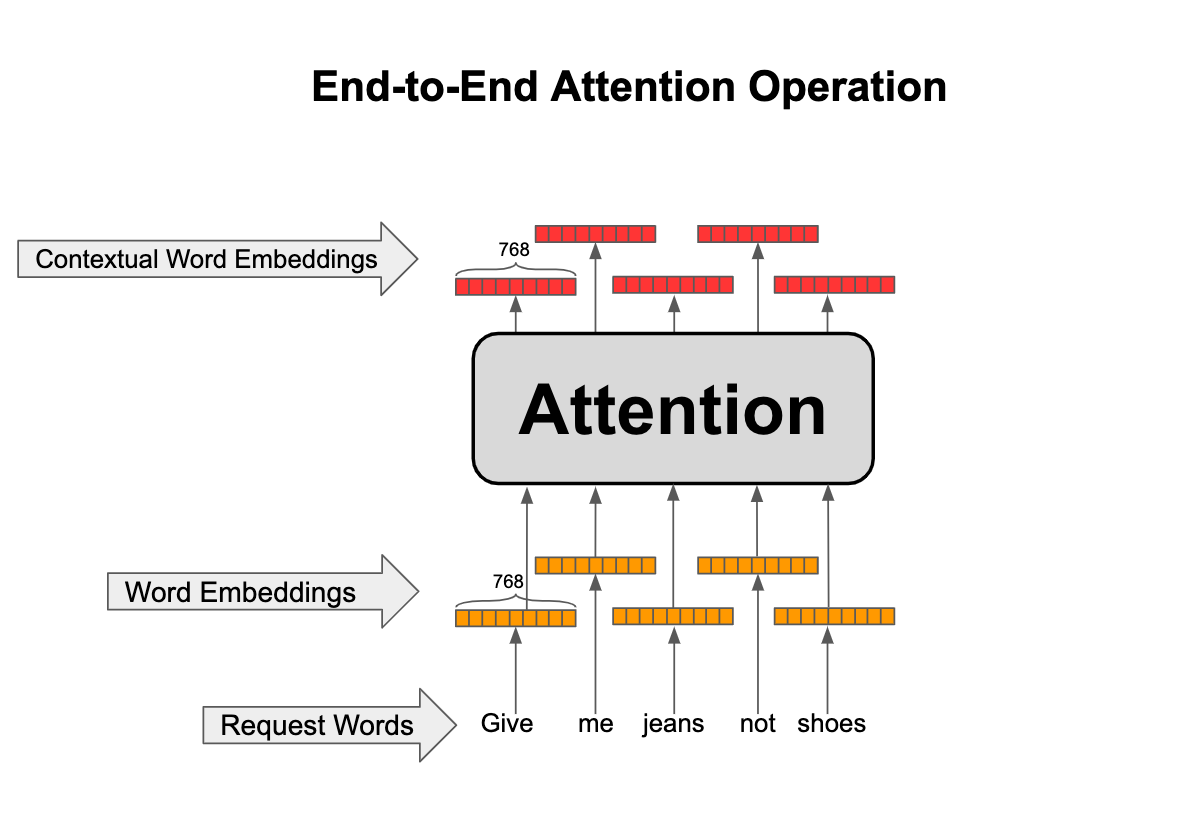
In the simplest form, the attention module does the following:
For each word in the input, it comes up with a contextualized embedding (with desired dimensionality, e.g., 768-dimensional) based on a weighted average of initial embeddings of all the words in the input as shown below. (We will show later how these contextualized embeddings are combined to result in a fixed-length vector.)
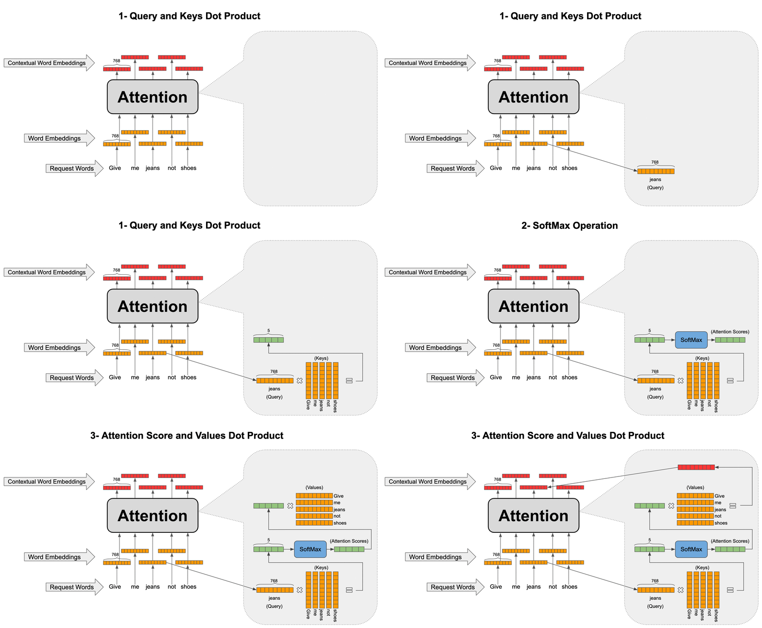
The attention operations go as shown in the animation below. For example, consider the word “jeans” and let’s see how the contextual representation is formed for this word:
- Let’s call “jeans” our query because we want to search for a contextual representation for it from the context. Take the embedding for “jeans” and multiply it by all the other word embeddings in the sentence (called keys) to find how similar or relevant they are to our query.
- Normalize the resulting five-dimensional vector (because our sentence has five words) by passing it through a SoftMax so that the sum of elements in the vector add up to one and call it attention scores.
- Attention scores are weights assigned to each word in the sentence when we want to fetch information about our query (“jeans” in this case) and now form a weighted average of the word embeddings in the sentence (called values) to construct the final contextual embedding for our query. You might think that values and keys are the same thing, but we are going to modify this basic attention mechanism next so that although they represent the same words, they are different representations of those words.
Multi-Head Attention
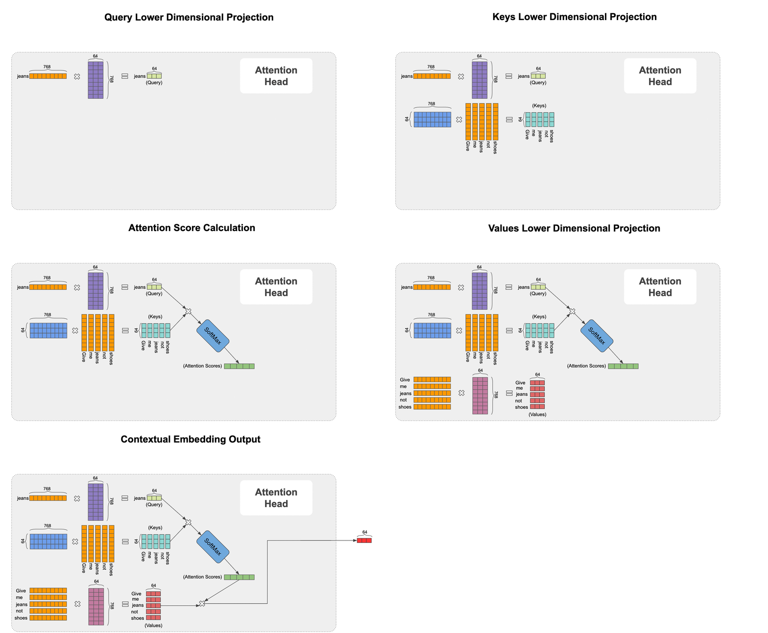
It’s time to introduce the multi-head attention concept. In this scheme, each query, key, and value is first projected into lower dimensional spaces and then the attention mechanism is applied. This projection is simply carried out by matrix-multiplying these vectors to different transformation matrices that are learned during training as seen in the animation below.
Next let’s combine the results of multiple different attention heads (e.g., 12) as shown below in a module called multi-head attention.
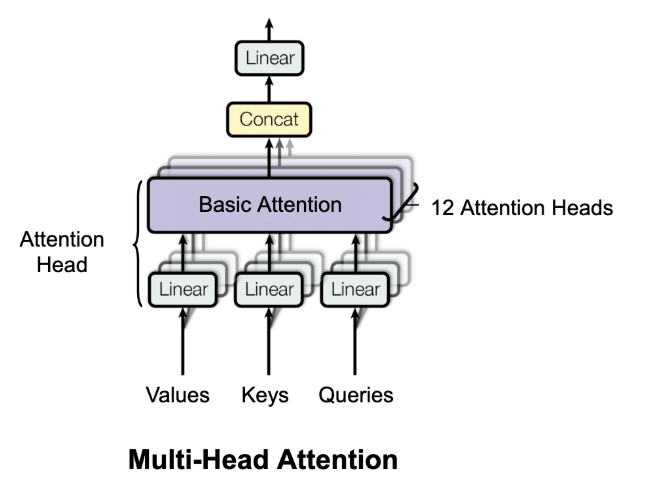
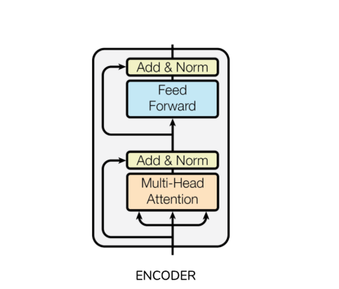
The logic behind this scheme is that each head can focus on a different linguistic concept (e.g., what is the relationship with the previous word or the next word?) and produce contextual embedding pertaining to that specific linguistic concept. Then a Transformer Encoder can be formed from a multi-head attention module as shown below.
BERT
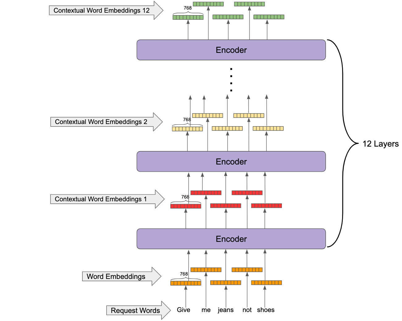
Finally, you get BERT which is simply a number of Transformer Encoders (e.g., 12) stacked on top of each other to get the output of the lower Encoder as input and produce a more sophisticated contextual embedding for each token as shown in the figure below. It’s worth noting that the initial word embeddings are fixed and learned during training but are summed up with different learned vectors based on their positions in the sentence. This way, the positional information is preserved.
In order to delve into the mechanics of how BERT works, this interactive notebook is very helpful. (Scroll to the last cell in the notebook.) You can choose to see how BERT employs the attention mechanism by investigating different attention heads in different layers of a trained BERT. Note that positive values are colored blue and negative values orange, with color intensity reflecting the magnitude of the value. Also, BERT makes use of some special tokens (more general than words) like [CLS] which is always added at the start of the input sequence, and [SEP] which comes at the end of the different segments of the input.
To see how BERT takes context into account as shown below, choose the 10th layer and 10th attention head and watch the attention scores when the query is “them.” It’s fascinating that in that head, the most attention is paid to “jeans” and “shoes,” but mostly to “shoes,” as “them” refers to shoes. You can see how the use of such a model that has a strong coreference resolution capability can help with our item selection problem.
Training BERT
It seems daunting to train such a huge network (in the basic form, it has 110 million parameters), but the good news is that Google has trained the network on all of English Wikipedia, so the model has a good understanding of the structure of English and its nuances. But, to really benefit from BERT, you have to finetune it on the desired task or a closely related task. Given the problem at hand, the next three stages of training are performed:
- Pre-training on Wikipedia data (done by Google):
- Mask a percentage of the words in the training data and maximize the likelihood of the most suitable tokens in the vocab to fill in the blanks based on the final contextual embedding of those masked tokens.
- Also follow training sentences with either random or observed next sentences and maximize the likelihood of detecting the correct next sentence from the final contextual embedding of the [CLS] special token.
- Take the pre-trained BERT from Google and use it as an initial point. Perform the same training as before using a large sample of our Fix Notes to help the model adapt to Fix Notes language. The way we used BERT for the third stage of training is shown in the figure below:
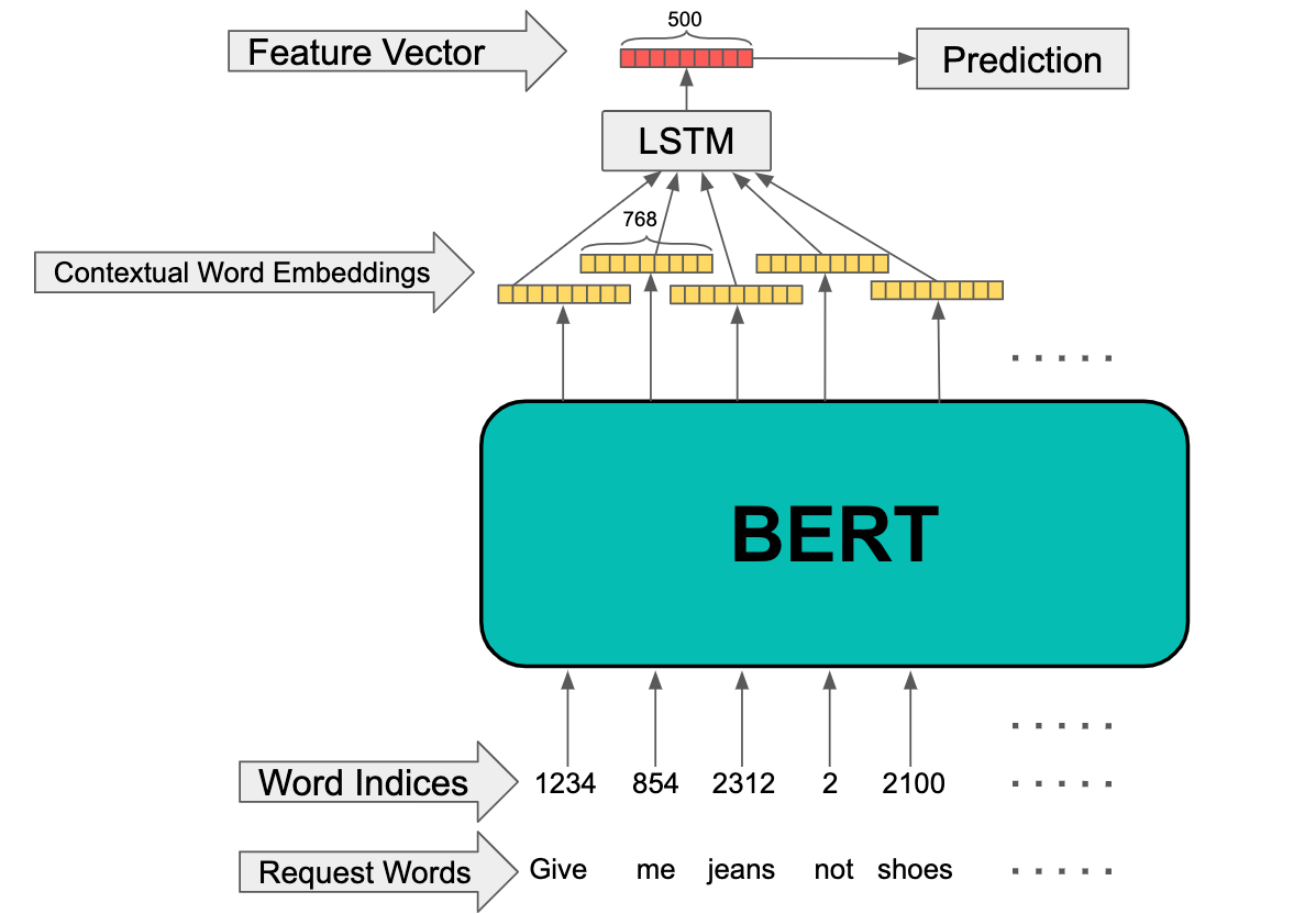
The final contextual embeddings (from the 12th layer of Transformer Encoders) for each token are fed to a bidirectional LSTM, and the final hidden state of the LSTM is used as the feature vector2. The resulting 500-dimensional vector can be thought of as a feature vector condensing the information contained in the request input.
- Define a new task as follows: Given a Fix Note, predict the probability of items in the inventory to be chosen by stylists based on the 500-dimensional feature vector of the request. For this task, the model shown above is used plus a SoftMax layer taking in the 500-dimensional feature vector to predict the probability of the items in the inventory3. The BERT module is initialized with the weights from the previous stage of training. Let’s take a look at one example of the results from the last stage of training:
Request: “I want black dresses. I really like what you sent before, so please more shorts like the last Fix, but no jeans.”
Top 5 most probable items:

Integration with Our Styling Model
The 500-dimensional feature vectors from the trained model (which can be thought of as high dimensional vectors summarizing the information in the Fix Notes) can now be fed into our styling algorithm which takes into account many different features about the client and items available. This imposes many different restrictions on the items that can be chosen, but at the same time unlocks many valuable gains because of the interaction of BERT features with other features related to the Fix. Let’s take a look at one example from the integration of BERT features into our styling model:
Request: “Can you please send me mildly fading skinny jean that has a good structure and is not ruined by one laundry visit. Going to Paris and would love a couple of floral blouses and a taupe open sweater. Also, I’m pretty busty these days, so nothing button down. My size right now is different from back when I signed up.”
8 most probable items:

As you can see, the BERT features captured this nuanced request surprisingly well, though not perfectly. The floral blouse and open sweater were surfaced, but not the skinny jeans. Fortunately, the stylist has the final say on how to best respect the request. Also, the request to avoid button downs is respected; if request features are not considered, the model would predict high probability for button-down items. In conclusion, attention-based models are state-of-the-art in many NLP tasks, and their usage in machine learning pipelines is rising despite their complexity. Hopefully, this post serves as a good introduction and motivation for those who want to integrate these models into their systems.
To read more about BERT and similar models, the following resources are recommended:
- BERT: Pre-training of Deep Bidirectional Transformers for Language Understanding
- Attention Is All You Need
- Cool illustrated explanation of BERT and Transformer
- Pytorch implementation of BERT repo
Footnotes
[1]↩ As of June 2019, BERT is no longer the state-of-the-art model and is dethroned by XLNet.
[2]↩ This scheme performs better than the use of [CLS] token’s contextual embedding as the feature vector.
[3]↩ In the case of our problem, training BERT simultaneously with the selection model does not perform as well as this scheme.
