At Stitch Fix, we love to test things. More broadly, in the tech community we love to test things. Is version A of the website better at converting users than version B? Do we make more money with version A of the recommendation engine than with version B?
We nearly always use the same vanilla framework for hypothesis testing that we were taught in Statistics 101.
\[\begin{align} H_0:& \mu_A - \mu_B = 0 \\ H_1:& \mu_A - \mu_B \neq 0 \\ \end{align}\]Although we rarely use the term, this test formulation is called a superiority trial. In this framework, we assume that there is no difference between the two means and we hold to that belief unless the data we have collected is strong enough to force us to reject it, demonstrating that one version (A or B) is superior to the other.
For many problems, the superiority trial is the right framework. We only want to rollout version B of the recommendation engine if it is demonstrably better than version A that is already in production. But for some problems, this is not the optimal approach. Consider the following examples:
- We are using a third party service to help us identify fraudulent credit cards. We’ve identified a different service that is substantially less expensive. If the less expensive service is just as good, we’d prefer to use that one. It doesn’t need to be better in order for us to switch.
- We have a need to deprecate a source of data (A) and replace it with a different one (B) for some system or model. We could delay deprecation of A if using B results in catastrophically bad outcomes, but sticking with A for the long haul is not an option.
- We would like to move from modeling approach A to modeling approach B, not because we expect better results with B but because it gives us more operational flexibility. We have no reason to believe B will be any worse but we wouldn’t want to make the move if it were.
- We have redesigned the website (version B) in a number of ways that we believe to be qualitatively superior than our current version A. We don’t expect differences in conversion or any of the key performance metrics on which we would typically evaluate the website but we believe there are benefits in dimensions that are either unmeasurable or that we lack the technology to measure.
In all of these cases, a superiority trial is not the best approach but it is very likely what most practitioners would do because it’s the default. We would (hopefully) diligently power our experiment to detect a reasonable effect size. If it were true that versions A and B performed very similarly, we may fail to reject the null hypothesis. Does that mean we can conclude that A and B essentially perform the same? No! Failing to reject the null hypothesis is not the same as accepting the null hypothesis.
Sample size calculations (which you definitely did 😉) are typically set up with more stringent bounds on a type I error (probability of falsely rejecting the null, often called alpha) than type II error (probability of failing to reject the null given that the null is false, often called beta). The typical value for alpha is 0.05 whereas the typical value for beta is 0.20, which corresponds to power = 0.80. That means we have a 20% chance of failing to detect a true effect of the magnitude that we stated in our power calculations, which is a pretty major blindspot. For a more relatable example, consider these hypotheses:
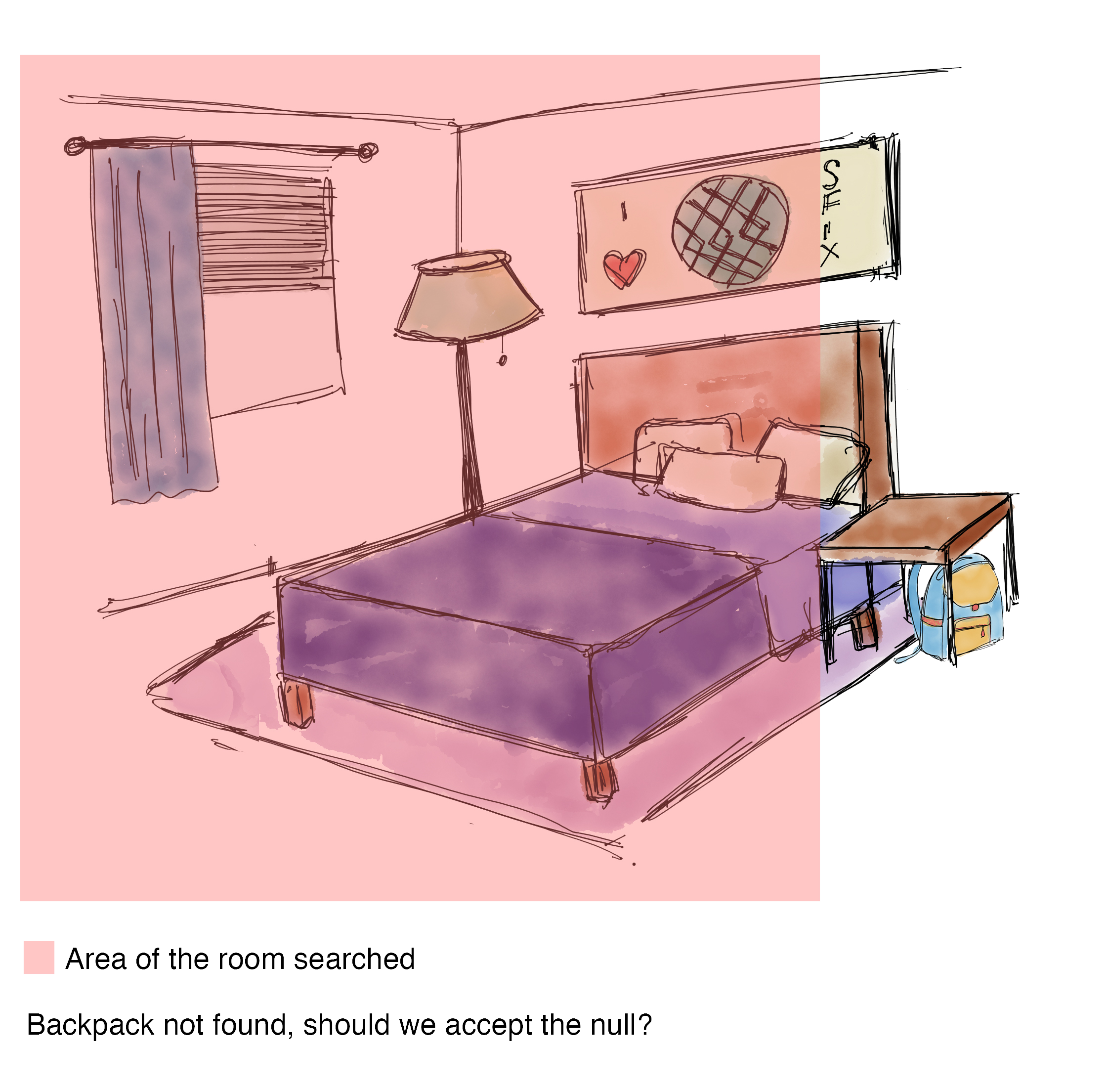
\[\begin{align} &H_0: \text{ my backpack is NOT in my room}\\ &H_1: \text{ my backpack IS in my room}\\ \end{align}\]If I search my room and find my backpack, cool I can reject the null. But if I search my room and don’t find my backpack (Figure 1), what should I think? Am I sure it isn’t there? Did I look hard enough? What if I only searched 80% of the room? It seems rash to conclude it definitely isn’t in there. No wonder we’re not allowed to “accept the null hypothesis,” whomp whomp.

So what’s a data scientist to do in this situation? You could increase your power a ton so you might feel better about failing to reject the null, but you would need a much larger sample size and the result still feels unsatisfying.
Luckily, there is a long history of problems like this in the clinical research world. Drug B is cheaper than Drug A, Drug B is expected to have fewer side-effects than Drug A, Drug B is easier to deliver because it doesn’t have to be refrigerated and Drug A does. Enter the non-inferiority trial. The non-inferiority trial is explicitly set up to demonstrate that version B is as good as version A, at least within some predetermined non-inferiority limit, \(\Delta\). We’ll talk more about how to set this limit in a minute but for now, assume that this is the minimal difference that is practically meaningful (usually called clinically significant in a clinical trial setting).
The hypotheses for a noninferiority trial flip our usual set-up on its head:
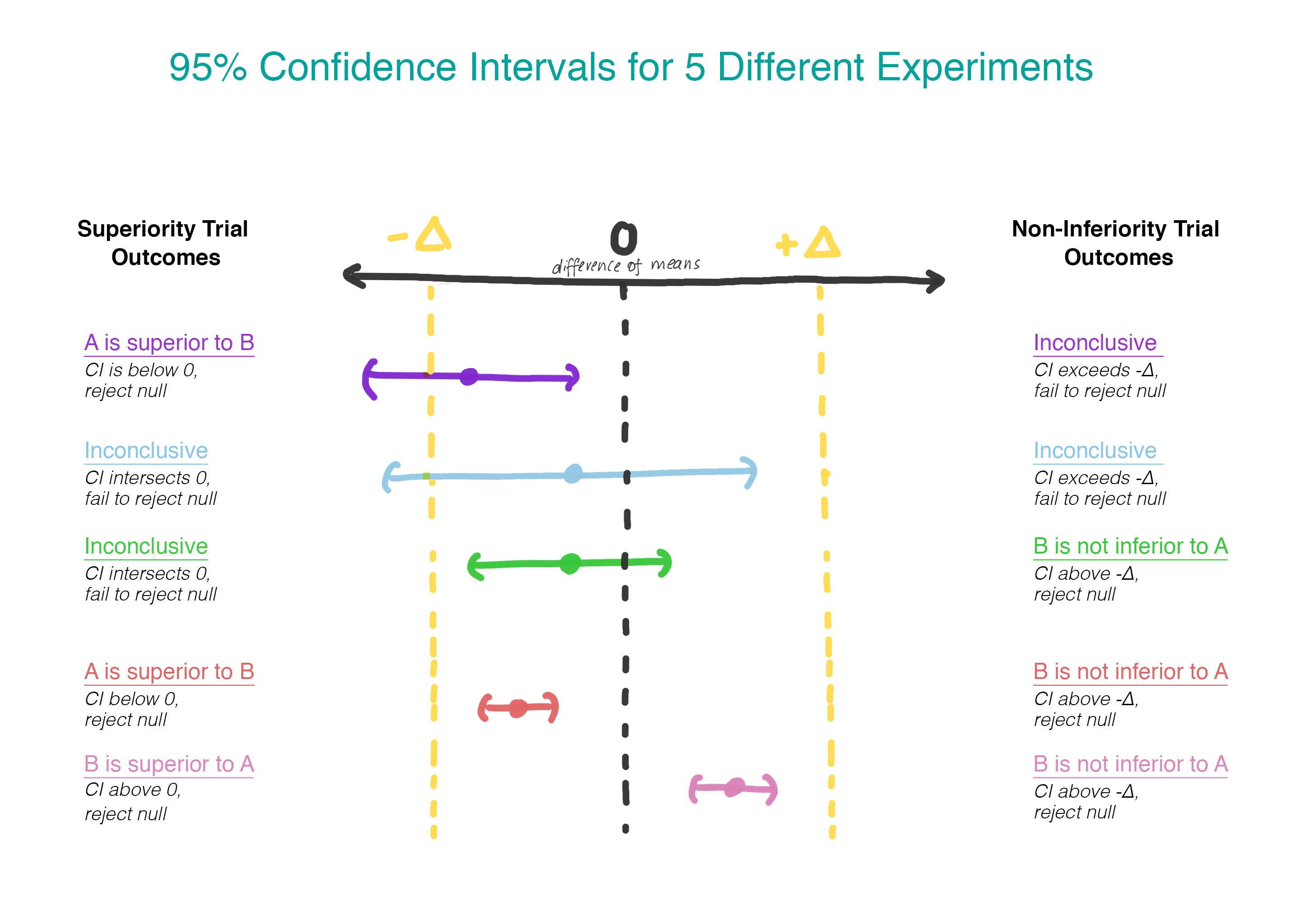
\[\begin{align} H_0:& \mu_B - \mu_A \leq - \Delta \\ H_1:& \mu_B - \mu_A > - \Delta \\ \end{align}\]Rather than assuming that there is no difference, now we are assuming that version B is worse than version A, and we will assume that until we can demonstrate that this is not the case. Finally, a moment where it makes sense to use a one-sided hypothesis test! Practically, this can be done by constructing a confidence interval and determining whether the interval is entirely greater than \(-\Delta\) (see Figure 2).

Choosing \(\Delta\)
How should one select \(\Delta\)? The selection of \(\Delta\) should be a mix of statistical reasoning and domain judgement. Regulatory guidance [1] in the clinical research world suggests the delta should be the smallest clinically relevant difference such that the difference would matter in practice. A quote from the European guidelines is a good gut check: “If an appropriate margin has been chosen, a confidence interval that lies entirely between –∆ and 0 … is still adequate to demonstrate non-inferiority. If this outcome does not seem acceptable, this demonstrates that ∆ has not been chosen appropriately.”
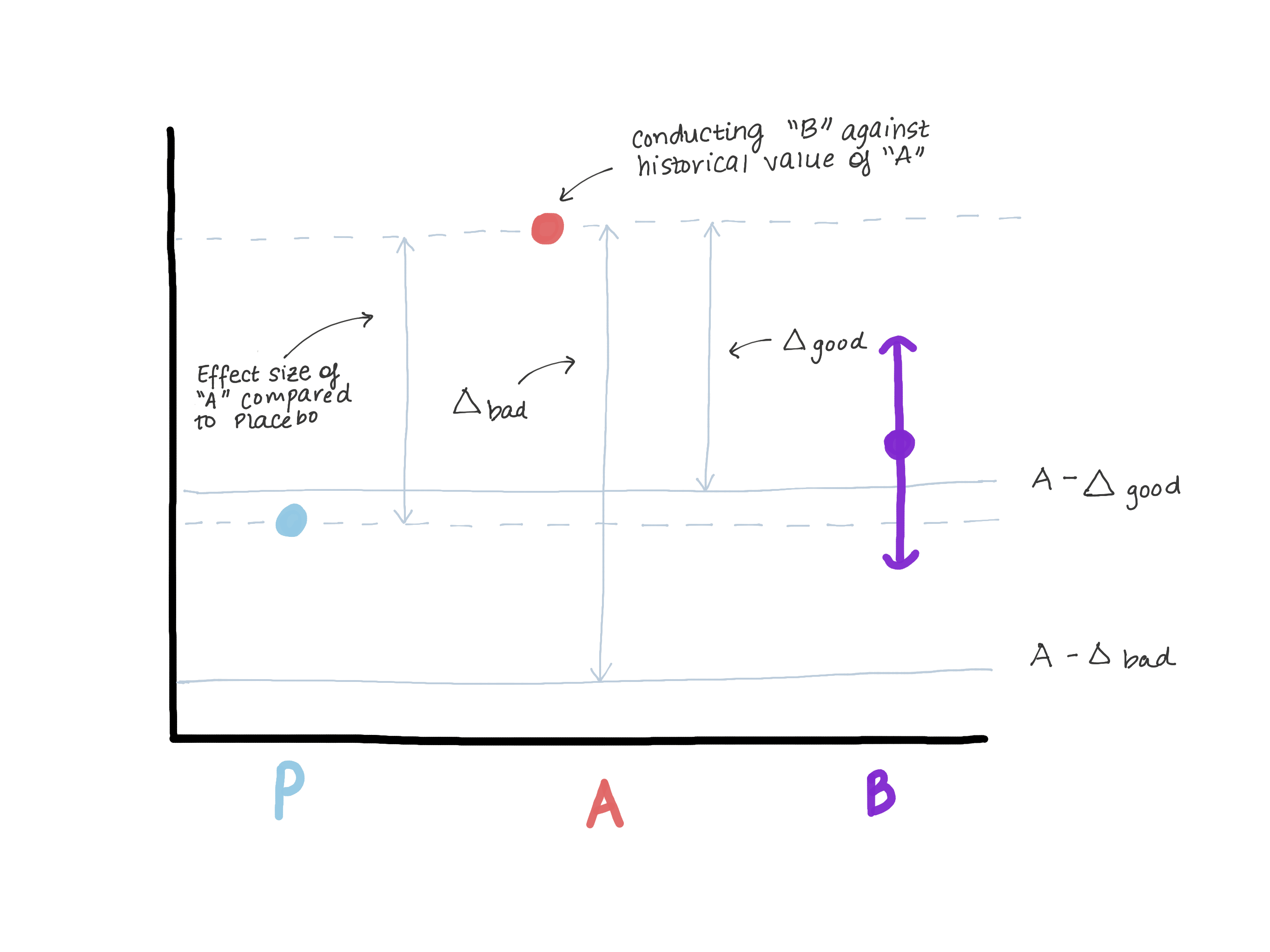
\(\Delta\) certainly should not exceed the magnitude of the effect of version A relative to a true control (placebo/no treatment) because that opens the door to version B being worse than the true control while still demonstrating “non-inferiority.” Suppose back in the day when version A was introduced, there was a version 0 in its place or the feature didn’t exist at all (see Figure 3). The superiority test that was performed that allowed version A to move into production found an effect size E (i.e., estimated \(\hat{\mu_A} - \hat{\mu_0} = E\)). Now A is our new normal and we’d like to make sure B is not inferior to A. Another way to write \(\mu_B - \mu_A \leq -\Delta\) (our null) is \(\mu_B \leq \mu_A - \Delta\). If we let \(\Delta\) be as big or bigger than E, then \(\mu_B \leq \mu_A - E \leq \text{Placebo}\). We may see that our estimate for \(\mu_B\) is entirely above \(\mu_A-E\), thereby rejecting the null and concluding that B is not inferior to A but at the same time, \(\mu_B\) could be \(\leq\) \(\mu_\text{placebo}\), which is not what we want (Figure 3).

Choosing \(\alpha\)
On to the sticky business of \(\alpha\). One could use the typical \(\alpha = 0.05\) and apply it all to one side, but that feels a little dirty, like when you’re buying something online and you stack discount codes that aren’t meant to be stacked except that the web developer made a mistake and you got away with it. Convention dictates that \(\alpha\) should be set at half the \(\alpha\) used in a superiority trial, i.e. \(0.05/2 = 0.025\), so take off those party hats.
Sample Size
What about sample size? If you believe that the true mean difference between A and B is 0, then the sample size calculation is the same as you would perform for a superiority test except that you’re replacing the effect size with the non-inferiority limit, assuming you’re using the \(\alpha_{\text{non-inferiority}} = \frac{1}{2}\alpha_{\text{superiority}}\). If you have reason to believe that B may be slightly worse than A but you want to demonstrate that it’s not \(\Delta\)-worse, then you’re in luck! That actually reduces your sample size because it’s easier to demonstrate that B is worse than A if you actually believe it to be a little worse, rather than equal.
A worked example
Suppose you would like to rollout version B barring evidence that it is more than 0.1 units worse than version A on a 5-point client-satisfaction outcome. You start by approaching this as a superiority test.
The typical sample size calculation we would do for a superiority trial would be the following:
\(\alpha = 0.05\), \(Z_{1-\alpha/2} = 1.96\)
\(\beta = 0.1\), power = 0.90, \(Z_{1-\beta}= 1.282\)
\(\sigma^2 = 1\) (estimated from data)
r = ratio of treatment to control, r = 1 for 1:1 or 50/50 allocation
\(\theta\) = effect size
\[\begin{align} N_{\text{per arm}} &= \frac{(r+1)(Z_{1-\beta} + Z_{1-\alpha/2})^2\sigma^2}{r\theta^2} \\ &= 2103 \\ \end{align}\]With 2,103 samples per arm, you’d be 90% confident that you would detect an effect of 0.10 or greater. But since you’re actually kind of worried about an effect as big as 0.10, maybe you don’t feel great powering your superiority study for that effect size. Maybe—to be on the safe side—you decide to power it for a smaller effect size, like 0.05. In that case, you’ll need 8,407 samples, a nearly 4-fold increase in sample size. But what if we stick with our original sample size but increase our power to 0.99 so we feel very confident detecting an effect if it is there? Then n per arm is 3,676 which is better but a more than 50% increase in sample size, and you’re still going to have to live with failing to reject the null rather than a result that definitively addresses your question.
What if, instead, you treated this as a non-inferiority trial? The sample size calculation is basically identical except for the denominator:
\[\begin{align} N_{\text{per arm}} = \frac{(r+1)(Z_{1-\beta} + Z_{1-\alpha})^2\sigma^2}{r((\mu_B - \mu_A) - \Delta)^2} \end{align}\]The following differ from the superiority formula:
- \(Z_{1-\alpha/2}\) is replaced with \(Z_{1-\alpha}\) but if you’re playing by the rules, you’ve replaced your \(\alpha = 0.05\) with \(\alpha = 0.025\), so these are actually the same number (1.96).
- \((\mu_B - \mu_A)\) appears in the denominator
- \(\theta\) (effect size) is replaced by \(\Delta\) (non-inferiority limit)
If we assume that \(\mu_B = \mu_A\), then \((\mu_B - \mu_A) = 0\) and the sample size calculation for a non-inferiority limit is exactly what we would have gotten with the superiority trial calculation for an effect size of 0.1. This is great! We can run the same size experiment with different hypotheses and a different approach to conclusions, and we get to answer the question we actually want to answer.
But wait, it gets better! Suppose that we don’t actually believe that \(\mu_B = \mu_A\); we think \(\mu_B\) is a little bit worse, maybe 0.01 units worse. That actually inflates our denominator, bringing down our sample size per arm to 1,737.
What happens if version B is actually an improvement over version A? We will reject the null hypothesis that B is worse than A by more than \(\Delta\) and accept the alternative hypothesis that B, if worse, is not worse by more than \(\Delta\) and may be better. Try writing that conclusion in a cross-functional presentation deck and see how it goes (seriously, I dare you). In a scenario where the longshot comes out a winner, no one wants to settle for “not worse by more than \(\Delta\) and maybe better.”
In this scenario, we can rely on the loquaciously named As Good As or Better Trial but could easily be called the equally loquacious Have Your Cake and Eat it Too Trial. This trial uses two sets of hypotheses:
First hypothesis set (same as non-inferiority trial):
\[\begin{align} H_0:& \mu_B - \mu_A \leq - \Delta \\ H_1:& \mu_B - \mu_A > - \Delta \\ \end{align}\]Second hypothesis set (same as superiority trial):
\[\begin{align} H_0:& \mu_B - \mu_A = 0 \\ H_1:& \mu_B - \mu_A \neq 0 \\ \end{align}\]If (and only if) the first null hypothesis is rejected, the second will be tested. By testing serially, we preserve the overall type I error rate (\(\alpha\)). Practically, this can be achieved by creating a 95% confidence interval for the difference in means and checking to see whether the entire interval exceeds \(-\Delta\). If it does not, we fail to reject the null and stop. If the entire interval does exceed \(-\Delta\), we continue on and see whether the interval contains 0, at which point the interpretation is the one we are used to from a vanilla superiority trial.
There is another type of trial, not yet discussed, called an equivalency trial. This term is often used interchangeably with a non-inferiority trial but in fact they have an important difference. While a non-inferiority trial is aiming to show that B is at least as good as A, an equivalency trial is aiming to show that B is at least as good as A and A is at least as good as B, which is harder. Practically, we are trying to determine whether the entire confidence interval for the difference in means lies between \(-\Delta\) and \(\Delta\). These trials require a greater sample size and have fewer practical applications in industry. So next time you are running an experiment in which your primary concern is making sure that the new version is not worse, don’t settle for “failing to reject the null.” Consider an alternate design to test the hypothesis that you actually care about.
This post heavily references material from:
Sample Sizes for Clinical Trials
Practical guide to sample size calculations: non-inferiority and equivalence trials
